Chapter 2 - Production (Python Code)

! pip install --upgrade quantecon_book_networks

Show code cell output Hide code cell output

Requirement already satisfied: quantecon_book_networks in /usr/share/miniconda3/envs/networks/lib/python3.11/site-packages (1.1)

Requirement already satisfied: numpy in /usr/share/miniconda3/envs/networks/lib/python3.11/site-packages (from quantecon_book_networks) (1.24.3)
Requirement already satisfied: scipy in /usr/share/miniconda3/envs/networks/lib/python3.11/site-packages (from quantecon_book_networks) (1.11.1)
Requirement already satisfied: pandas in /usr/share/miniconda3/envs/networks/lib/python3.11/site-packages (from quantecon_book_networks) (2.0.3)
Requirement already satisfied: matplotlib in /usr/share/miniconda3/envs/networks/lib/python3.11/site-packages (from quantecon_book_networks) (3.7.2)
Requirement already satisfied: pandas-datareader in /usr/share/miniconda3/envs/networks/lib/python3.11/site-packages (from quantecon_book_networks) (0.10.0)
Requirement already satisfied: networkx in /usr/share/miniconda3/envs/networks/lib/python3.11/site-packages (from quantecon_book_networks) (3.1)
Requirement already satisfied: quantecon in /usr/share/miniconda3/envs/networks/lib/python3.11/site-packages (from quantecon_book_networks) (0.7.1)
Requirement already satisfied: POT in /usr/share/miniconda3/envs/networks/lib/python3.11/site-packages (from quantecon_book_networks) (0.9.3)
Requirement already satisfied: contourpy>=1.0.1 in /usr/share/miniconda3/envs/networks/lib/python3.11/site-packages (from matplotlib->quantecon_book_networks) (1.0.5)
Requirement already satisfied: cycler>=0.10 in /usr/share/miniconda3/envs/networks/lib/python3.11/site-packages (from matplotlib->quantecon_book_networks) (0.11.0)
Requirement already satisfied: fonttools>=4.22.0 in /usr/share/miniconda3/envs/networks/lib/python3.11/site-packages (from matplotlib->quantecon_book_networks) (4.25.0)
Requirement already satisfied: kiwisolver>=1.0.1 in /usr/share/miniconda3/envs/networks/lib/python3.11/site-packages (from matplotlib->quantecon_book_networks) (1.4.4)
Requirement already satisfied: packaging>=20.0 in /usr/share/miniconda3/envs/networks/lib/python3.11/site-packages (from matplotlib->quantecon_book_networks) (23.1)
Requirement already satisfied: pillow>=6.2.0 in /usr/share/miniconda3/envs/networks/lib/python3.11/site-packages (from matplotlib->quantecon_book_networks) (9.4.0)
Requirement already satisfied: pyparsing<3.1,>=2.3.1 in /usr/share/miniconda3/envs/networks/lib/python3.11/site-packages (from matplotlib->quantecon_book_networks) (3.0.9)
Requirement already satisfied: python-dateutil>=2.7 in /usr/share/miniconda3/envs/networks/lib/python3.11/site-packages (from matplotlib->quantecon_book_networks) (2.8.2)

Requirement already satisfied: pytz>=2020.1 in /usr/share/miniconda3/envs/networks/lib/python3.11/site-packages (from pandas->quantecon_book_networks) (2023.3.post1)
Requirement already satisfied: tzdata>=2022.1 in /usr/share/miniconda3/envs/networks/lib/python3.11/site-packages (from pandas->quantecon_book_networks) (2023.3)
Requirement already satisfied: lxml in /usr/share/miniconda3/envs/networks/lib/python3.11/site-packages (from pandas-datareader->quantecon_book_networks) (4.9.3)
Requirement already satisfied: requests>=2.19.0 in /usr/share/miniconda3/envs/networks/lib/python3.11/site-packages (from pandas-datareader->quantecon_book_networks) (2.31.0)

Requirement already satisfied: numba>=0.49.0 in /usr/share/miniconda3/envs/networks/lib/python3.11/site-packages (from quantecon->quantecon_book_networks) (0.57.1)
Requirement already satisfied: sympy in /usr/share/miniconda3/envs/networks/lib/python3.11/site-packages (from quantecon->quantecon_book_networks) (1.11.1)

Requirement already satisfied: llvmlite<0.41,>=0.40.0dev0 in /usr/share/miniconda3/envs/networks/lib/python3.11/site-packages (from numba>=0.49.0->quantecon->quantecon_book_networks) (0.40.0)
Requirement already satisfied: six>=1.5 in /usr/share/miniconda3/envs/networks/lib/python3.11/site-packages (from python-dateutil>=2.7->matplotlib->quantecon_book_networks) (1.16.0)

Requirement already satisfied: charset-normalizer<4,>=2 in /usr/share/miniconda3/envs/networks/lib/python3.11/site-packages (from requests>=2.19.0->pandas-datareader->quantecon_book_networks) (2.0.4)
Requirement already satisfied: idna<4,>=2.5 in /usr/share/miniconda3/envs/networks/lib/python3.11/site-packages (from requests>=2.19.0->pandas-datareader->quantecon_book_networks) (3.4)
Requirement already satisfied: urllib3<3,>=1.21.1 in /usr/share/miniconda3/envs/networks/lib/python3.11/site-packages (from requests>=2.19.0->pandas-datareader->quantecon_book_networks) (1.26.16)
Requirement already satisfied: certifi>=2017.4.17 in /usr/share/miniconda3/envs/networks/lib/python3.11/site-packages (from requests>=2.19.0->pandas-datareader->quantecon_book_networks) (2023.7.22)
Requirement already satisfied: mpmath>=0.19 in /usr/share/miniconda3/envs/networks/lib/python3.11/site-packages (from sympy->quantecon->quantecon_book_networks) (1.3.0)

We begin with some imports.

import quantecon as qe
import quantecon_book_networks
import quantecon_book_networks.input_output as qbn_io
import quantecon_book_networks.plotting as qbn_plt
import quantecon_book_networks.data as qbn_data
ch2_data = qbn_data.production()
default_figsize = (6, 4)
export_figures = False

import numpy as np
import pandas as pd
import networkx as nx
import matplotlib.pyplot as plt
import matplotlib.cm as cm
import matplotlib.colors as plc
from matplotlib import cm
quantecon_book_networks.config("matplotlib")

Multisector Models

We start by loading a graph of linkages between 15 US sectors in 2021.

Our graph comes as a list of sector codes, an adjacency matrix of sales between the sectors, and a list the total sales of each sector.

In particular, Z[i,j] is the sales from industry i to industry j, and X[i] is the the total sales of each sector i.

codes = ch2_data["us_sectors_15"]["codes"]
Z = ch2_data["us_sectors_15"]["adjacency_matrix"]
X = ch2_data["us_sectors_15"]["total_industry_sales"]

Now we define a function to build coefficient matrices.

Two coefficient matrices are returned. The backward linkage case, where sales between sector i and j are given as a fraction of total sales of sector j. The forward linkage case, where sales between sector i and j are given as a fraction of total sales of sector i.

def build_coefficient_matrices(Z, X):
    """
    Build coefficient matrices A and F from Z and X via 
    
        A[i, j] = Z[i, j] / X[j] 
        F[i, j] = Z[i, j] / X[i]
    
    """
    A, F = np.empty_like(Z), np.empty_like(Z)
    n = A.shape[0]
    for i in range(n):
        for j in range(n):
            A[i, j] = Z[i, j] / X[j]
            F[i, j] = Z[i, j] / X[i]

    return A, F

A, F = build_coefficient_matrices(Z, X)

Backward linkages for 15 US sectors in 2021

Here we calculate the hub-based eigenvector centrality of our backward linkage coefficient matrix.

centrality = qbn_io.eigenvector_centrality(A)

Now we use the quantecon_book_networks package to produce our plot.

fig, ax = plt.subplots(figsize=(8, 10))
plt.axis("off")
color_list = qbn_io.colorise_weights(centrality, beta=False)
# Remove self-loops
A1 = A.copy()
for i in range(A1.shape[0]):
    A1[i][i] = 0
qbn_plt.plot_graph(A1, X, ax, codes, 
              layout_type='spring',
              layout_seed=5432167,
              tol=0.0,
              node_color_list=color_list) 

if export_figures:
    plt.savefig("figures/input_output_analysis_15.pdf")
plt.show()

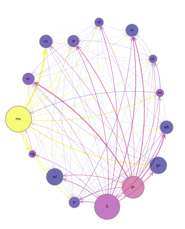
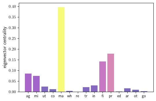
Eigenvector centrality of across US industrial sectors

Now we plot a bar chart of hub-based eigenvector centrality by sector.

fig, ax = plt.subplots(figsize=default_figsize)
ax.bar(codes, centrality, color=color_list, alpha=0.6)
ax.set_ylabel("eigenvector centrality", fontsize=12)
if export_figures:
    plt.savefig("figures/input_output_analysis_15_ec.pdf")
plt.show()

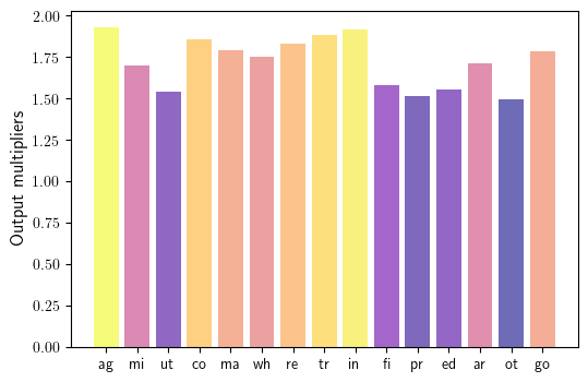
Output multipliers across 15 US industrial sectors

Output multipliers are equal to the authority-based Katz centrality measure of the backward linkage coefficient matrix.

Here we calculate authority-based Katz centrality using the quantecon_book_networks package.

omult = qbn_io.katz_centrality(A, authority=True)

fig, ax = plt.subplots(figsize=default_figsize)
omult_color_list = qbn_io.colorise_weights(omult,beta=False)
ax.bar(codes, omult, color=omult_color_list, alpha=0.6)
ax.set_ylabel("Output multipliers", fontsize=12)
if export_figures:
    plt.savefig("figures/input_output_analysis_15_omult.pdf")
plt.show()

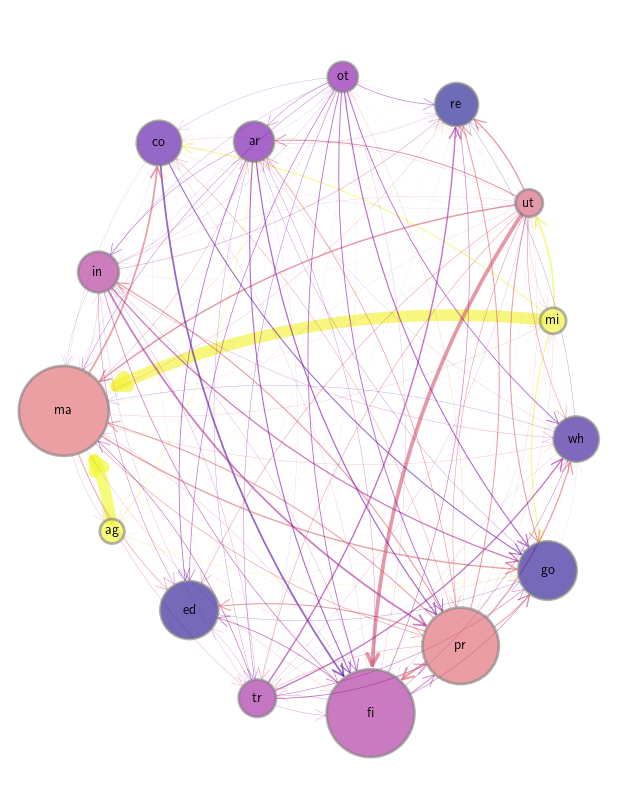
Forward linkages and upstreamness over US industrial sectors

Upstreamness is the hub-based Katz centrality of the forward linkage coefficient matrix.

Here we calculate hub-based Katz centrality.

upstreamness = qbn_io.katz_centrality(F)

Now we plot the network.

fig, ax = plt.subplots(figsize=(8, 10))
plt.axis("off")
upstreamness_color_list = qbn_io.colorise_weights(upstreamness,beta=False)
# Remove self-loops
for i in range(F.shape[0]):
    F[i][i] = 0
qbn_plt.plot_graph(F, X, ax, codes, 
              layout_type='spring', # alternative layouts: spring, circular, random, spiral
              layout_seed=5432167,
              tol=0.0,
              node_color_list=upstreamness_color_list) 

if export_figures:
    plt.savefig("figures/input_output_analysis_15_fwd.pdf")
plt.show()

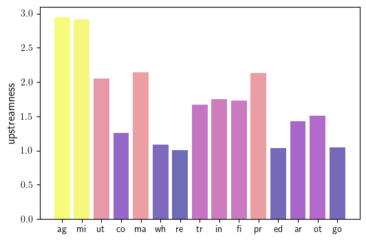
Relative upstreamness of US industrial sectors

Here we produce a barplot of upstreamness.

fig, ax = plt.subplots(figsize=default_figsize)
ax.bar(codes, upstreamness, color=upstreamness_color_list, alpha=0.6)
ax.set_ylabel("upstreamness", fontsize=12)
if export_figures:
    plt.savefig("figures/input_output_analysis_15_up.pdf")
plt.show()

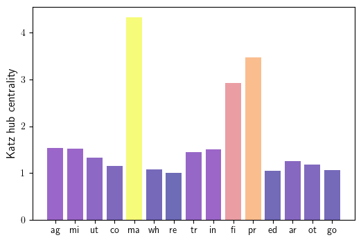
Hub-based Katz centrality of across 15 US industrial sectors

Next we plot the hub-based Katz centrality of the backward linkage coefficient matrix.

kcentral = qbn_io.katz_centrality(A)

fig, ax = plt.subplots(figsize=default_figsize)
kcentral_color_list = qbn_io.colorise_weights(kcentral,beta=False)
ax.bar(codes, kcentral, color=kcentral_color_list, alpha=0.6)
ax.set_ylabel("Katz hub centrality", fontsize=12)
if export_figures:
    plt.savefig("figures/input_output_analysis_15_katz.pdf")
plt.show()

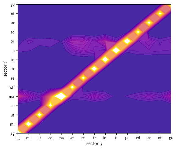
The Leontief inverse 𝐿 (hot colors are larger values)

We construct the Leontief inverse matrix from 15 sector adjacency matrix.

I = np.identity(len(A))
L = np.linalg.inv(I - A)

Now we produce the plot.

fig, ax = plt.subplots(figsize=(6.5, 5.5))

ticks = range(len(L))

levels = np.sqrt(np.linspace(0, 0.75, 100))

co = ax.contourf(ticks, 
                    ticks,
                    L,
                    levels,
                    alpha=0.85, cmap=cm.plasma)

ax.set_xlabel('sector $j$', fontsize=12)
ax.set_ylabel('sector $i$', fontsize=12)
ax.set_yticks(ticks)
ax.set_yticklabels(codes)
ax.set_xticks(ticks)
ax.set_xticklabels(codes)

if export_figures:
    plt.savefig("figures/input_output_analysis_15_leo.pdf")
plt.show()

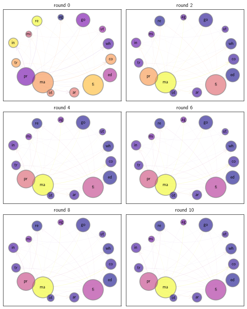
Propagation of demand shocks via backward linkages

We begin by generating a demand shock vector \(d\).

N = len(A)
np.random.seed(1234)
d = np.random.rand(N) 
d[6] = 1  # positive shock to agriculture

Now we simulate the demand shock propagating through the economy.

sim_length = 11
x = d
x_vecs = []
for i in range(sim_length):
    if i % 2 ==0:
        x_vecs.append(x)
    x = A @ x

Finally, we plot the shock propagating through the economy.

fig, axes = plt.subplots(3, 2, figsize=(8, 10))
axes = axes.flatten()

for ax, x_vec, i in zip(axes, x_vecs, range(sim_length)):
    if i % 2 != 0:
        pass
    ax.set_title(f"round {i*2}")
    x_vec_cols = qbn_io.colorise_weights(x_vec,beta=False)
    # remove self-loops
    for i in range(len(A)):
        A[i][i] = 0
    qbn_plt.plot_graph(A, X, ax, codes,
                  layout_type='spring',
                  layout_seed=342156,
                  node_color_list=x_vec_cols,
                  node_size_multiple=0.00028,
                  edge_size_multiple=0.8)

plt.tight_layout()
if export_figures:
    plt.savefig("figures/input_output_analysis_15_shocks.pdf")
plt.show()

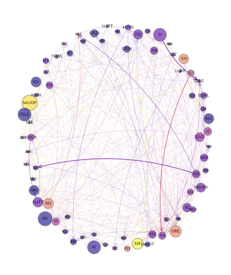
Network for 71 US sectors in 2021

We start by loading a graph of linkages between 71 US sectors in 2021.

codes_71 = ch2_data['us_sectors_71']['codes']
A_71 = ch2_data['us_sectors_71']['adjacency_matrix']
X_71 = ch2_data['us_sectors_71']['total_industry_sales']

Next we calculate our graph’s properties.

We use hub-based eigenvector centrality as our centrality measure for this plot.

centrality_71 = qbn_io.eigenvector_centrality(A_71)
color_list_71 = qbn_io.colorise_weights(centrality_71,beta=False)

Finally we produce the plot.

fig, ax = plt.subplots(figsize=(10, 12))
plt.axis("off")
# Remove self-loops
for i in range(A_71.shape[0]):
    A_71[i][i] = 0
qbn_plt.plot_graph(A_71, X_71, ax, codes_71,
              node_size_multiple=0.0005,
              edge_size_multiple=4.0,
              layout_type='spring',
              layout_seed=5432167,
              tol=0.01,
              node_color_list=color_list_71)

if export_figures:
    plt.savefig("figures/input_output_analysis_71.pdf")
plt.show()

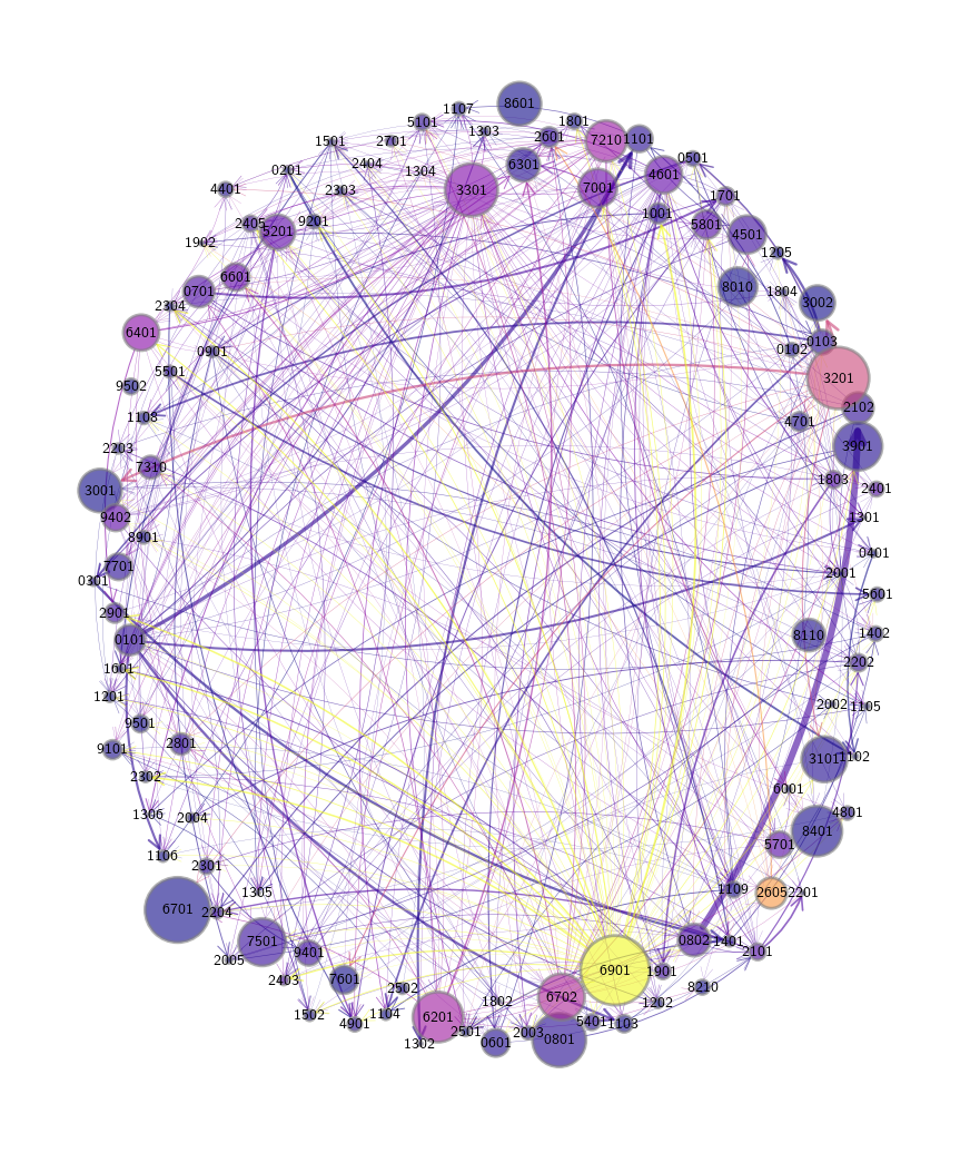
Network for 114 Australian industry sectors in 2020

Next we load a graph of linkages between 114 Australian sectors in 2020.

codes_114 = ch2_data['au_sectors_114']['codes']
A_114 = ch2_data['au_sectors_114']['adjacency_matrix']
X_114 = ch2_data['au_sectors_114']['total_industry_sales']

Next we calculate our graph’s properties.

We use hub-based eigenvector centrality as our centrality measure for this plot.

centrality_114 = qbn_io.eigenvector_centrality(A_114)
color_list_114 = qbn_io.colorise_weights(centrality_114,beta=False)

Finally we produce the plot.

fig, ax = plt.subplots(figsize=(11, 13.2))
plt.axis("off")
# Remove self-loops
for i in range(A_114.shape[0]):
    A_114[i][i] = 0
qbn_plt.plot_graph(A_114, X_114, ax, codes_114,
              node_size_multiple=0.008,
              edge_size_multiple=5.0,
              layout_type='spring',
              layout_seed=5432167,
              tol=0.03,
              node_color_list=color_list_114)

if export_figures:
    plt.savefig("figures/input_output_analysis_aus_114.pdf")
plt.show()

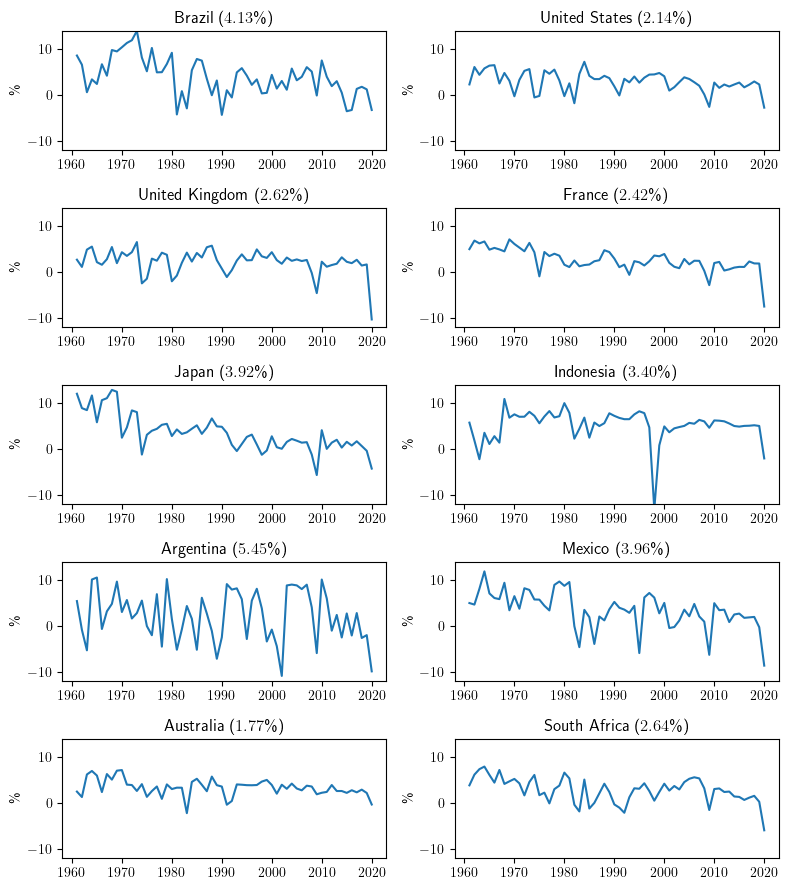
GDP growth rates and std. deviations (in parentheses) for 8 countries

Here we load a pandas DataFrame of GDP growth rates.

gdp_df = ch2_data['gdp_df']
gdp_df.head()

country	Brazil	United States	United Kingdom	France	Japan	Indonesia	Argentina	Mexico	Australia	South Africa
year
1961	8.6	2.3	2.677119	4.980112	12.043536	5.740646	5.427843	5.000000	2.482618	3.844734
1962	6.6	6.1	1.102910	6.843470	8.908973	1.841978	-0.852022	4.664415	1.294258	6.177931
1963	0.6	4.4	4.874384	6.233680	8.473642	-2.237030	-5.308197	8.106887	6.216364	7.373709
1964	3.4	5.8	5.533659	6.652100	11.676708	3.529698	10.130298	11.905481	6.980438	7.939609
1965	2.4	6.4	2.142177	4.861508	5.819708	1.081589	10.569433	7.100000	5.980351	6.122798

Now we plot the growth rates and calculate their standard deviations.

fig, axes = plt.subplots(5, 2, figsize=(8, 9))
axes = axes.flatten()

countries = gdp_df.columns
t = np.asarray(gdp_df.index.astype(float))
series = [np.asarray(gdp_df[country].astype(float)) for country in countries]


for ax, country, gdp_data in zip(axes, countries, series):
    
    ax.plot(t, gdp_data)
    ax.set_title(f'{country} (${gdp_data.std():1.2f}$\%)' )
    ax.set_ylabel('\%')
    ax.set_ylim((-12, 14))

plt.tight_layout()
if export_figures:
    plt.savefig("figures/gdp_growth.pdf")
plt.show()