Chapter 3 - Optimal Flows (Julia Code)

Bellman’s Method

Here we demonstrate solving a shortest path problem using Bellman’s method.

Our first step is to set up the cost function, which we store as an array called c. Note that we set c[i, j] = Inf when no edge exists from i to j.

c = fill(Inf, (7, 7))
c[1, 2], c[1, 3], c[1, 4] = 1, 5, 3
c[2, 4], c[2, 5] = 9, 6
c[3, 6] = 2
c[4, 6] = 4
c[5, 7] = 4
c[6, 7] = 1
c[7, 7] = 0

Next we define the Bellman operator.

function T(q)
    Tq = similar(q)
    n = length(q)
    for x in 1:n
        Tq[x] = minimum(c[x, :] + q[:])
    end
    return Tq
end

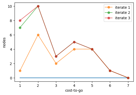
Now we arbitrarily set \(q \equiv 0\), generate the sequence of iterates \(T_q\), \(T^2_q\), \(T^3_q\) and plot them. By \(T^3_q\) has already converged on \(q^∗\).

using PyPlot
export_figures = false
fig, ax = plt.subplots(figsize=(6, 4))

n = 7
q = zeros(n)
ax.plot(1:n, q)
ax.set_xlabel("cost-to-go")
ax.set_ylabel("nodes")

for i in 1:3
    new_q = T(q)
    ax.plot(1:n, new_q, "-o", alpha=0.7, label="iterate $i")
    q = new_q
end

ax.legend()
if export_figures == true
    plt.savefig("figures/shortest_path_iter_1.pdf")
end

Linear programming

When solving linear programs, one option is to use a domain specific modeling language to set out the objective and constraints in the optimization problem. Here we demonstrate the Julia package JuMP.

using JuMP
using GLPK

We create our model object and select our solver.

m = Model()
set_optimizer(m, GLPK.Optimizer)

Now we add variables, constraints and an objective to our model.

@variable(m, q1 >= 0)
@variable(m, q2 >= 0)
@constraint(m, 2q1 + 5q2 <= 30)
@constraint(m, 4q1 + 2q2 <= 20)
@objective(m, Max, 3q1 + 4q2)

Finally we solve our linear program.

optimize!(m)

println(value.(q1)) 
println(value.(q2))

2.5
5.0